Design an Ad Click Event Aggregation System
Most systems in this series can lose a little data and survive. A dropped metric leaves a gap on a chart. A missed location update is corrected 30 seconds later.
This one is different, and the difference changes everything: these numbers become invoices.
Ad click aggregation decides how much advertisers pay and how much publishers earn. A 1% error on a billion clicks a day is millions of dollars, in someone’s favour, every month. That single fact is why this design reaches for exactly-once processing — which we spent the last chapter establishing is expensive and usually unnecessary.
Here it is necessary. That makes this the design where the expensive option is the correct one.
Step 1 — Scope
Requirements
Input: log files on many servers, appended with each click. Each event has ad_id, click_timestamp, user_id, ip, country.
Three queries to support:
- Number of clicks for a given
ad_idin the last M minutes. - The top 100 most clicked ads in the past minute — both parameters configurable.
- Filtering by
ip,user_idorcountryon either of the above.
Edge cases explicitly in scope: events arriving late, duplicate events, and partial system failure.
Latency: a few minutes end-to-end is fine.
That last one deserves attention, because it’s easy to misread. Real-time bidding operates in under a second — an auction runs while the page loads. But aggregation is for billing and reporting, and nobody needs their spend dashboard accurate to the second.
Being handed a relaxed latency budget is a gift, and it should be spent. Those minutes are what buy room for watermarks, deduplication, and exactly-once machinery. A system with a one-second budget could not be correct in the same way.
Back-of-the-envelope
- 1 billion ad clicks per day, 2 million ads total
- Growth: 30% year over year — traffic doubles about every three years
Click QPS = 10⁹ / 10⁵ = 10,000
Peak QPS (5×)          = 50,000
Storage = 0.1 KB × 10⁹ = 100 GB/day ≈ 3 TB/month
Note the shape of this: 50,000 QPS is a serious write load, but 3 TB a month is nothing. The difficulty is throughput and correctness, not volume.
Step 2 — High-level design
The query API
The client here is a dashboard, and the requirements name exactly two questions it asks:
| Endpoint | Answers |
|---|---|
GET /v1/ads/{ad_id}/aggregated_count | How many clicks did this ad get in the last M minutes? |
GET /v1/ads/popular_ads | Which N ads were clicked most in the last M minutes? |
Both take from and to minute bounds — defaulting to the last minute — and both take a filter identifier rather than free-form filter expressions. 001 might mean “non-US clicks”.
That last choice looks like a limitation and is actually the design. Arbitrary filtering means arbitrary aggregation at query time, which is what this whole pipeline exists to avoid. A fixed set of filter identifiers means each one can be pre-aggregated, and the query stays a lookup. It reappears as the star schema below.
Two kinds of data
Raw events — every click, as it happened:
ad_id    click_timestamp        user_id   ip              country
ad001    2021-01-01 00:00:01    user1     207.148.22.22   USA
ad001    2021-01-01 00:00:02    user1     207.148.22.22   USA
ad002    2021-01-01 00:00:02    user2     209.153.56.11   USA
Aggregated data — counts per ad per minute:
| ad_id | click_minute | filter_id | count |
|---|---|---|---|
| ad001 | 202101010000 | 0012 | 2 |
| ad001 | 202101010000 | 0023 | 3 |
Keep both. Aggregated data is what you query — the raw form is far too large to scan for every dashboard refresh. But raw data is the backup you compute from when the aggregation is wrong, and aggregation logic will eventually be wrong. Old raw data moves to cold storage; aggregated data stays hot.
That’s the whole argument for keeping raw events, and it’s the same instinct as an append-only log: a derived value can always be rebuilt from a source of truth, and never the other way round.
Filtering with a star schema
Requirement three — filter by country, IP, user — is handled by pre-aggregating along each dimension:
| ad_id | click_minute | country | count |
|---|---|---|---|
| ad001 | 202101010001 | USA | 100 |
| ad001 | 202101010001 | GBR | 200 |
| ad001 | 202101010001 | others | 3000 |
This is a star schema, standard in data warehousing, and the filtering fields are dimensions. Queries are fast because every answer is precomputed.
The cost is combinatorial: each new dimension multiplies the number of rows. If that sounds familiar, it’s the same multiplication as the cardinality problem in the last chapter — precomputed aggregates and time-series labels blow up for identical reasons.
The pipeline
A synchronous pipeline would be fragile. If producers outrun consumers — a traffic spike, a slow node — consumers run out of memory, and one failed component stops everything.
Two message queues fix that:
flowchart TD
    LW["Log watcher
tails click logs"] --> Q1{{"Message queue 1
raw click events"}}
    Q1 --> AGG["Aggregation service
map · aggregate · reduce"]
    Q1 --> DW1["Database writer"]
    DW1 --> RAW[("Raw data DB
Cassandra")]
    AGG --> Q2{{"Message queue 2
per-minute counts
+ top-N"}}
    Q2 --> DW2["Database writer"]
    DW2 --> AGGDB[("Aggregation DB")]
    AGGDB --> QS["Query service
dashboards"]

    style Q1 fill:#fce7f3,stroke:#db2777,color:#831843
    style Q2 fill:#fce7f3,stroke:#db2777,color:#831843
    style AGG fill:#dbeafe,stroke:#2563eb,color:#1e3a8a
    style RAW fill:#f1f5f9,stroke:#64748b,color:#334155
Why a second queue rather than writing results straight to the database? Because the boundary between “aggregation finished” and “result durably stored” is exactly where exactly-once guarantees are won or lost. A queue that supports atomic commit lets the aggregator commit its output and its input offset together. Writing directly to a database splits that into two operations that can disagree.
The aggregation service as a DAG
Aggregation is a MapReduce-shaped problem, expressed as a directed acyclic graph:
flowchart LR
    IN["Click events"] --> M["Map
clean, normalise,
partition by ad_id"]
    M --> A1["Aggregate
count per ad, per minute
(in memory)"]
    M --> A2["Aggregate"]
    M --> A3["Aggregate"]
    A1 --> R["Reduce
merge partial top-N
into global top-N"]
    A2 --> R
    A3 --> R
    R --> OUT["Results"]

    style M fill:#dcfce7,stroke:#16a34a,color:#14532d
    style A1 fill:#dbeafe,stroke:#2563eb,color:#1e3a8a
    style A2 fill:#dbeafe,stroke:#2563eb,color:#1e3a8a
    style A3 fill:#dbeafe,stroke:#2563eb,color:#1e3a8a
    style R fill:#fce7f3,stroke:#db2777,color:#831843
Why a Map node at all? You could partition in Kafka and let aggregators subscribe directly. Two reasons not to: input often needs cleaning or normalising first, and you may not control how events were produced — so events for the same ad_id can land in different partitions. The Map node re-partitions on a key you actually chose.
Top-N reduces beautifully. Each aggregator keeps a heap of its own top 3. The reducer takes 3 candidates from each of 3 nodes — 9 total — and picks the global top 3. Each node ships a tiny summary rather than its full counts, which is what makes the whole approach scale.
Step 3 — Deep dive
Event time or processing time?
The most important decision in this design, and it is not close.
Event time is when the click happened. Processing time is when your server got round to it.
They diverge — sometimes enormously. A phone goes through a tunnel and its event arrives five hours late.
| Advantage | Problem | |
|---|---|---|
| Event time | Results are correct — the click genuinely happened then | Depends on a client-supplied clock, which may be wrong or forged |
| Processing time | The server’s clock is reliable | A delayed event is counted in the wrong minute |
Use event time. When the output is an invoice, a click must be billed to the minute it occurred, not the minute your pipeline noticed. Processing time produces results that are reliably computed and wrong.
Which creates the problem that defines every streaming system: if you aggregate by event time, when do you stop waiting?
Watermarks
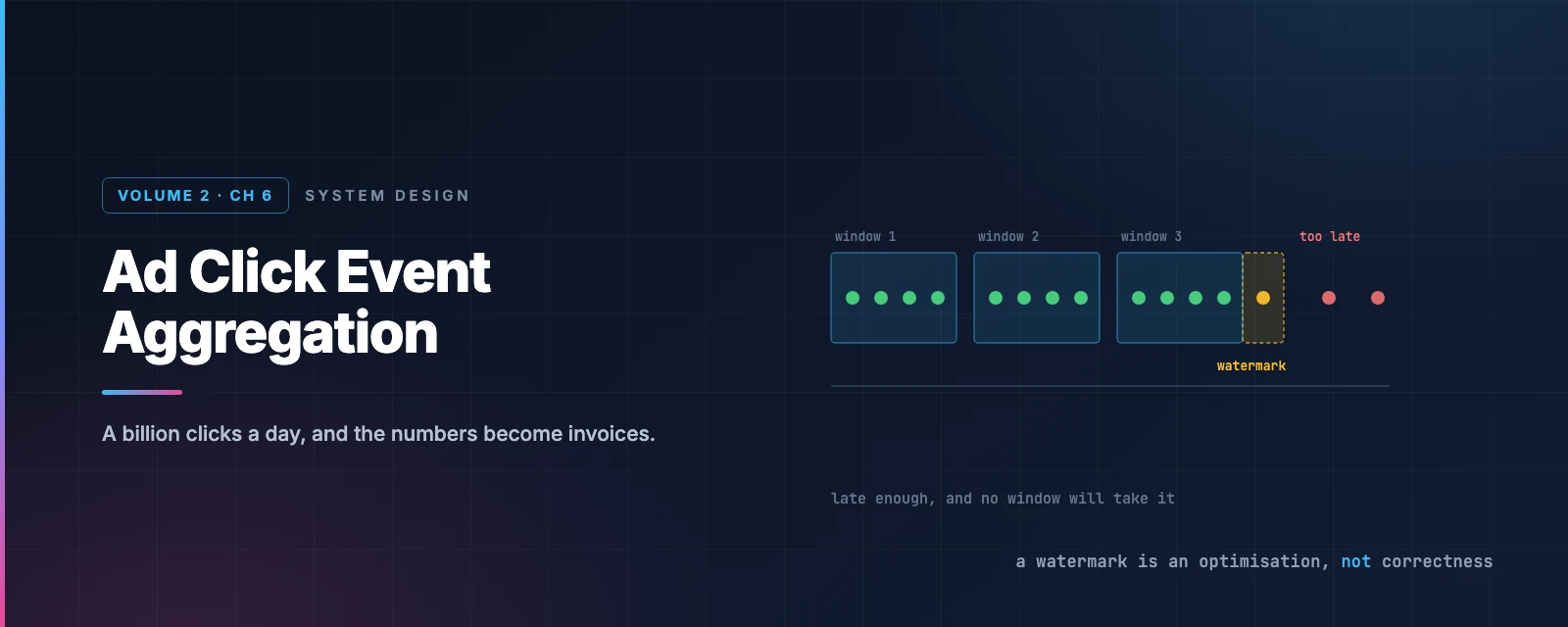
A minute-long window covering 00:00–00:01 could theoretically receive a matching event at any point in the future. Wait forever and you never emit a result. Close at 00:01 and you lose every event still in flight.
A watermark extends the window by a grace period. Close the 00:00–00:01 window at 00:01:15 and events up to 15 seconds late still land correctly.
The dial is pure trade-off:
- A long watermark catches more late events — more accuracy, more latency.
- A short watermark emits sooner — less latency, less accuracy.
Find the right watermark
Below is a fixed set of clicks, each with a real arrival delay. The distribution is realistic: most events are nearly instant, a handful lag by tens of seconds, and two are hopelessly late. Drag the watermark and watch what you buy:
Two lessons come out of dragging that slider.
Every second you wait buys progressively less. With no watermark you land 9 of 16 events in the right window — you lose even the ones only a second or two late, because they were unlucky enough to click near the end of the minute. Fifteen seconds gets you to 11. A full minute gets you to 14.
Then it stops. Push the slider to 120 seconds and you still get 14. Events o and p are 15 minutes and 5 hours late, and no watermark you would ever accept reaches them — waiting five hours to close a one-minute window is absurd. The curve flattens hard, and where it flattens is where you stop paying.
So watermarks are explicitly not a correctness mechanism — they’re a cheap way to capture the bulk of lateness. Genuine correctness comes from somewhere else.
Reconciliation
That somewhere else is a nightly batch job that re-reads the raw events, sorts them by event time, and compares its totals against what the streaming pipeline produced.
There’s no third party to reconcile against — unlike banking, where you compare your ledger to the bank’s. So the check is the same data computed a different way: a slow, complete, order-insensitive batch pass against a fast, approximate, streaming one.
That is the actual answer to late events. The watermark catches 95% cheaply. Reconciliation catches the rest, slowly, and corrects the record before anyone is billed.
Windows
Tumbling windows are fixed-length and non-overlapping — 00:00–00:01, 00:01–00:02. Right for “clicks per minute”, since every event belongs to exactly one window.
Sliding windows overlap: “top ads in the last 3 minutes”, recomputed every minute. Right for query two, where the window is longer than the update interval.
flowchart TD
    subgraph T["Tumbling — count per minute"]
        T1["00:00–00:01"] --- T2["00:01–00:02"] --- T3["00:02–00:03"]
    end
    subgraph S["Sliding — top-N over 3 min, every min"]
        S1["00:00–00:03"]
        S2["00:01–00:04"]
        S3["00:02–00:05"]
    end

    style T fill:#dbeafe,stroke:#2563eb,color:#1e3a8a
    style S fill:#dcfce7,stroke:#16a34a,color:#14532d
Exactly-once, and why it’s genuinely hard
Duplicates come from two places: clients resending (malicious repetition is a fraud problem, not an aggregation one), and server failure mid-aggregation.
The failure case is the instructive one. An aggregator consumes offsets 100–110, aggregates them, sends the result downstream, then commits offset 110 upstream. If it dies after sending but before committing, a replacement starts again at 100 — and those clicks are billed twice.
The obvious fixes each fail:
Save the offset to external storage before processing? Then if the send fails, the offset says 110 and those events are never processed at all. You traded duplication for loss.
Save the offset after the downstream acknowledges? Better — but the gap between “downstream acked” and “offset saved” is still a window where a crash duplicates.
sequenceDiagram
    autonumber
    participant U as Upstream Kafka
    participant A as Aggregator
    participant D as Downstream Kafka

    U->>A: poll from offset 100
    Note over A: aggregate 100 to 110
    A->>D: send aggregated result
    D-->>A: ack
    Note over A,D: crash here and offsets 100 to 110
are sent twice — clicks billed twice
    A->>U: commit offset 110
You cannot close the gap by reordering two operations. Whichever you do first, a crash between them produces either loss or duplication. The only real fix is to make the send and the commit one atomic transaction — which is why the second message queue exists, and why the design needs a system that supports distributed transactions.
Exactly-once isn’t a setting. It’s a transaction boundary drawn around two operations that must agree.
Scaling, and the hotspot
The three components — queue, aggregation, database — are decoupled and scale independently.
Partition by ad_id so all events for one ad land in one partition and one aggregator. Pre-allocate partitions generously: changing the partition count remaps ad IDs to different partitions, which scrambles in-flight aggregation state.
Which creates the problem this design has and the previous ones didn’t: hotspots.
Ad traffic is extremely skewed. A company with a multi-million-dollar budget generates orders of magnitude more clicks than a local shop. Partitioning by ad_id sends all of that to one node.
The fix is dynamic: when a node exceeds capacity, it requests more resources, splits its events across additional nodes, and the partial results are merged back.
flowchart TD
    HOT["ad1 — 300 events
node capacity is 100"] -->|"1 · request resources"| RM["Resource manager"]
    RM -->|"2 · allocate"| N1["Aggregator A · 100"]
    RM --> N2["Aggregator B · 100"]
    RM --> N3["Aggregator C · 100"]
    N1 -->|"4 · merge"| RED["Reduce"]
    N2 --> RED
    N3 --> RED

    style HOT fill:#fee2e2,stroke:#dc2626,color:#7f1d1d
    style RED fill:#dcfce7,stroke:#16a34a,color:#14532d
Partition keys that are natural are often skewed. ad_id is the obvious key and the skewed one. Detecting hot keys and splitting them dynamically is the general answer — the same shape as the celebrity problem in the news feed chapter.
Fault tolerance
Aggregation happens in memory, so a node crash loses its counts. You can replay from Kafka — but replaying from the beginning is impossibly slow.
Snapshot the state periodically: not just the upstream offset, but the aggregation state itself — the running counts and the top-N heaps. On failure, a new node loads the latest snapshot and replays only the events after it.
Lambda or Kappa?
The design has two processing paths: streaming for live results, batch for historical replay and reconciliation. That’s Lambda architecture, and its well-known flaw is two codebases computing the same thing — which drift, and disagree in ways nobody can explain.
Kappa architecture uses one path. Reprocessing history means replaying old events through the same streaming engine.
This design is Kappa: recalculation reads raw data and pushes it through a dedicated instance of the same aggregation service, so live traffic isn’t disturbed but the logic is identical. One implementation, two data sources.
If two paths must agree, make them literally the same code. Anything else is a reconciliation problem you invented for yourself.
What has changed since the book
Flink’s checkpointing is the mechanism this needs
“Wrap it in a distributed transaction” is where most treatments stop, filing the rest under advanced topics. It’s worth knowing how stream processors actually do it.
Flink implements a variant of the Chandy-Lamport distributed snapshot algorithm called asynchronous barrier snapshotting. The job manager injects barriers into the source streams. Barriers flow along with the data; when an operator has received the barrier on all its inputs, it snapshots its state and forwards the barrier downstream. When every operator acknowledges, the checkpoint is complete.
That gives a consistent cut across a distributed pipeline without stopping it.
End-to-end exactly-once then needs transactional sinks: the sink writes inside a transaction and commits nothing until the checkpoint completes. A crash rolls the transaction back and the pipeline restarts from the last checkpoint — the two-phase commit described above, built into the framework.
This is the practical answer to that unwinnable ordering problem: don’t hand-roll it. Use an engine where the transaction boundary is part of the execution model.
Real-time OLAP databases took over the serving layer
ClickHouse and Druid are often listed as an alternative. They’ve become the mainstream answer.
Columnar, real-time OLAP stores — Druid, ClickHouse, Apache Pinot — ingest streaming data and serve aggregate queries over billions of rows in milliseconds. They absorb both jobs the design splits between an aggregation service and an aggregation database: ingest the stream, pre-aggregate on the way in, serve slice-and-dice queries.
That collapses much of the architecture. You still need the streaming layer for exactly-once and windowing, but the star-schema tables and the query service become one system.
The industry tried to make this obsolete — and failed
The most interesting development, and it goes well beyond architecture.
This entire design assumes you can identify and count clicks across sites. That assumption came under sustained attack: Apple’s App Tracking Transparency, browsers blocking third-party cookies, and Google’s Privacy Sandbox — launched 2019 to replace cookie-based measurement with privacy-preserving APIs.
The Attribution Reporting API was the replacement for exactly what this design builds. Rather than a log of individual clicks, it offered aggregated, deliberately noisy reports: summary reports processed through an aggregation service that returns only noisy aggregates, and event-level reports carrying just 3 bits of conversion data for a click, 1 bit for a view, delivered with deliberate delay. Differential privacy applied to ad measurement.
It did not survive.
- July 2024 — Google reversed course and said it would not deprecate third-party cookies.
- April 2025 — the replacement plan, a user prompt, was dropped too.
- October 2025 — Google retired ten Privacy Sandbox APIs, Attribution Reporting among them, citing “low levels of adoption” alongside sustained regulatory pressure. Chrome began deprecating them in Chrome 144 and targeted removal for Chrome 150.
A smaller set survives — CHIPS, FedCM, Private State Tokens — chosen for having actually been adopted.
Two things worth taking from that.
The design above is not obsolete. A platform counting clicks on its own inventory — the first-party case — is unaffected by any of this, and that is precisely what’s designed here. What the privacy work targeted was cross-site attribution.
And the industry attempted to replace exact counting with statistically noisy aggregates, deliberately trading accuracy for privacy — the exact opposite of the premise here, that a 1% error is millions of dollars. It’s a striking example of a non-technical requirement reshaping an architecture, and of an ambitious redesign failing not on engineering merit but on adoption.
What to take away
Correctness requirements come from what the output is used for. Metrics tolerate loss because a gap in a chart is survivable. Clicks don’t, because they become invoices. Ask what the number does before choosing a delivery guarantee — the answer determines whether exactly-once is worth its cost.
Event time versus processing time is the fundamental streaming decision. Processing time is easy and produces confidently wrong answers. Event time is correct and forces you to decide when to stop waiting — which is the whole discipline of watermarks and windows.
Watermarks are an optimisation, not a correctness mechanism. They cheaply catch the bulk of lateness. The genuinely late tail is unreachable at any acceptable latency, so correctness comes from a batch reconciliation pass, not a longer wait.
Exactly-once is a transaction boundary, not a config value. Sending downstream and committing an offset must be atomic. Reorder them all you like — a crash in the gap gives you loss one way and duplication the other.
Natural partition keys are usually skewed. ad_id is the obvious key, and a handful of advertisers dwarf everyone else. Expect hot keys and plan to split them; the alternative is one overloaded node while the rest idle.
Keep the raw data. Aggregates are derived, and derived values are eventually wrong. Raw events are what let you recompute after the bug is fixed — which is also what makes reconciliation possible at all.
References and Further Reading
Stream processing
- Flink fault tolerance — checkpoints, barriers and exactly-once
- Data streaming fault tolerance — asynchronous barrier snapshotting in detail
- The Chandy–Lamport algorithm — the 1985 paper Flink's checkpointing derives from
- Apache Flink · Spark Streaming
- Designing Data-Intensive Applications — Chapter 11 on stream processing and window types
Analytics stores
- ClickHouse · Apache Druid · Apache Pinot
- Apache Cassandra
- Apache Parquet · Apache ORC · Apache Avro
- Star schema
Architecture patterns
- Lambda architecture · Questioning the Lambda Architecture — Jay Kreps's original Kappa argument
- Apache Hadoop YARN
Advertising and privacy
- Attribution Reporting API — the privacy-preserving replacement, now being retired
- Privacy Sandbox — the initiative's history and its retirement
- Real-time bidding · Click-through rate
- On the Differential Privacy and Interactivity of Privacy Sandbox Reports
In this series
- The complete guide — every article in order
- Design a Distributed Message Queue — delivery semantics, and what exactly-once costs
- Metrics Monitoring and Alerting — the same aggregation shape where loss is acceptable
- Design a News Feed System — the other design ruined by skewed keys