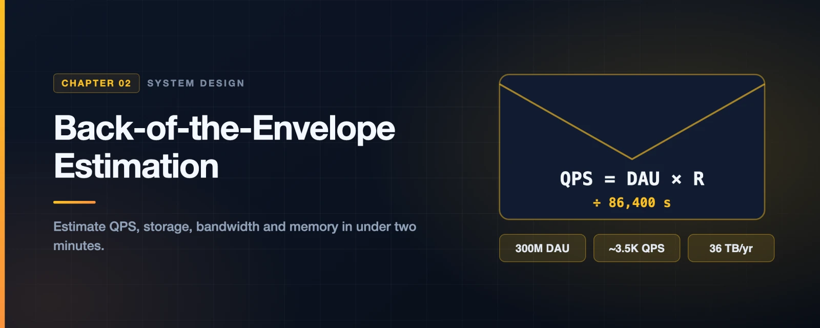
Back-of-the-Envelope Estimation: The Art of Making Smart Guesses
Imagine your interviewer says: “We’re designing Instagram Stories. How much storage do we need per year?”
Most junior engineers freeze. They don’t know where to begin. They feel like they need exact numbers — the real database size, the real compression ratios, the real usage stats.
Here’s the secret: you are not supposed to be exact. You are supposed to be directionally correct.
Back-of-the-envelope estimation is the skill of producing a reasonable answer in 2–3 minutes using simple math and a handful of memorized numbers. Google’s Jeff Dean calls it:
“Estimates you create using a combination of thought experiments and common performance numbers to get a good feel for which designs will meet your requirements.”
This skill separates engineers who guess from engineers who reason from numbers. Let’s build it from the ground up.
Why This Skill Matters
Before any system design, you need to answer three questions:
- How much traffic will hit my servers? (QPS — queries per second)
- How much data will I store? (Storage)
- How fast does each component need to be? (Latency)
Without answers to these, you’re guessing at architecture. With them, you can make decisions like:
- “We need a CDN because our image reads are 50,000/sec”
- “One database can handle this — we don’t need sharding yet”
- “This operation touches disk — it’ll be too slow, we need a cache”
Foundation 1: The Power of Two — How Big Is Your Data?
All data in computers is stored in bytes. A byte is 8 bits, and one ASCII character is one byte. When you deal with distributed systems the volumes get enormous, but the arithmetic still comes back to a handful of multiples.
Strictly speaking, data volume is defined in powers of two:
| Power | Approximate value | Full name | Short name |
|---|---|---|---|
| 2^10 | 1 thousand | 1 Kilobyte | 1 KB |
| 2^20 | 1 million | 1 Megabyte | 1 MB |
| 2^30 | 1 billion | 1 Gigabyte | 1 GB |
| 2^40 | 1 trillion | 1 Terabyte | 1 TB |
| 2^50 | 1 quadrillion | 1 Petabyte | 1 PB |
A precision note most sources skip. 2^10 is 1,024 bytes, not 1,000. The strictly correct name for 1,024 bytes is a kibibyte (KiB); “kilobyte” formally means 1,000 bytes. Storage vendors sell you decimal GB, while your operating system reports binary GiB — which is exactly why a “1 TB” drive shows up as about 931 GB.
For estimation, ignore all of that and use powers of ten. Here is the version you actually calculate with:
1 KB  =  1,000 bytes         (10^3)   ← a short text message
1 MB  =  1,000,000 bytes     (10^6)   ← a 1-minute MP3 song
1 GB  =  1,000,000,000 bytes (10^9)   ← a 2-hour HD movie
1 TB  =  10^12 bytes                  ← 1,000 HD movies
1 PB  =  10^15 bytes                  ← Netflix's daily data volume
graph LR
    B[1 Byte
a single char] -->|×1,000| KB[1 KB
a tweet]
    KB -->|×1,000| MB[1 MB
a photo]
    MB -->|×1,000| GB[1 GB
a movie]
    GB -->|×1,000| TB[1 TB
1,000 movies]
    TB -->|×1,000| PB[1 PB
whole Netflix]

    style B fill:#6366F1,stroke:#4338CA,color:#fff
    style KB fill:#3B82F6,stroke:#1D4ED8,color:#fff
    style MB fill:#10B981,stroke:#047857,color:#fff
    style GB fill:#F59E0B,stroke:#B45309,color:#fff
    style TB fill:#EF4444,stroke:#B91C1C,color:#fff
    style PB fill:#8B5CF6,stroke:#6D28D9,color:#fff
Real-world anchor points
| Object | Size |
|---|---|
| A single character (ASCII) | 1 byte |
| An integer (32-bit) | 4 bytes |
| A tweet (280 chars) | ~280 bytes |
| A profile photo (compressed) | ~300 KB |
| A high-res photo | 3–5 MB |
| A 4K video minute | ~350 MB |
| 1 million user rows in a DB | ~1 GB |
Tip: In estimates, treat 1 KB ≈ 1,000 bytes, not 1,024. The 2.4% error is irrelevant for rough estimates. Keep the math simple.
Foundation 2: Latency Numbers — How Fast Is Fast?
This is the single most important table in system design. Memorize the order of magnitude for each operation. Originally measured by Dr. Jeff Dean at Google in 2010, the relative order still holds.
Operation                              Time
───────────────────────────────────────────────────────
L1 cache reference                     0.5 ns
Branch mispredict                      5 ns
L2 cache reference                     7 ns
Mutex lock/unlock                      100 ns
Main memory reference (RAM)            100 ns
─ ─ ─ ─ ─ ─ ─ ─ ─ ─ ─ ─ ─ ─ ─ ─ ─ ─ ─ ─ ─ ─ ─ ─
Compress 1 KB with Zippy               10,000 ns  = 10 μs
Send 2 KB over 1 Gbps network          20,000 ns  = 20 μs
Read 1 MB sequentially from memory    250,000 ns  = 250 μs
Round trip within same datacenter     500,000 ns  = 500 μs
─ ─ ─ ─ ─ ─ ─ ─ ─ ─ ─ ─ ─ ─ ─ ─ ─ ─ ─ ─ ─ ─ ─ ─
Disk seek (HDD)                    10,000,000 ns  = 10 ms
Read 1 MB sequentially from network 10,000,000 ns = 10 ms
Read 1 MB sequentially from disk    30,000,000 ns = 30 ms
─ ─ ─ ─ ─ ─ ─ ─ ─ ─ ─ ─ ─ ─ ─ ─ ─ ─ ─ ─ ─ ─ ─ ─
Send packet CA → Netherlands → CA  150,000,000 ns = 150 ms
What has changed since 2010 (and what has not)
Dean’s table is from 2010 and is still what interviewers expect you to quote. But one line in it is now badly out of date, and knowing which one is a genuine edge.
The disk line. In 2010, “disk” meant a spinning platter and a seek cost ~10 ms. Today a production database sits on NVMe flash, where a random 4 KB read is roughly 20 µs. That is not an improvement — it is about three orders of magnitude, and it changes conclusions:
| Operation | 2010 (HDD) | 2026 (NVMe) | Change |
|---|---|---|---|
| Random read | ~10 ms | ~20 µs | ~500× faster |
| Read 1 MB sequentially | ~30 ms | ~50 µs | ~600× faster |
| Same-datacenter round trip | ~500 µs | ~500 µs | unchanged |
| Main memory reference | ~100 ns | ~80 ns | roughly flat |
| CA → Netherlands → CA | ~150 ms | ~150 ms | unchanged, and never will |
Read that table by column, not by row. The interesting fact is not that flash got fast — it is that storage got 500× faster while the network did not move at all. A round trip across a datacenter is now slower than reading a megabyte off local disk, which was unthinkable in 2010.
What this means for design:
- “Avoid disk, it’s slow” is a 2010 heuristic. On NVMe, an extra disk read is often cheaper than an extra network hop.
- The network is the new disk. Chattiness between services — the N+1 query across a service boundary — is now the dominant cost in most systems.
- The one number that has not improved and cannot is the speed of light. San Francisco to Amsterdam is ~150 ms round trip because physics says so. No amount of engineering removes it; only moving the data closer does, which is the entire argument for CDNs and multi-region deployments.
- Memory is still roughly 250× faster than NVMe, so caching still wins. It just wins by a smaller margin than the classic table implies.
In an interview, quoting Dean’s numbers is correct and expected. Adding “though NVMe has closed the memory-to-disk gap by about three orders of magnitude since then” is what makes you sound like someone who has actually operated a system.
Visualizing the gap — the “zoom out” perspective
The difference between a cache hit and a disk seek is hard to grasp in nanoseconds. Here’s a human-scale analogy:
If 1 ns = 1 second, then...

L1 Cache          │█│                        0.5 seconds
RAM               │██████████│               100 seconds (1.6 min)
SSD read          │████████████████████│     ~150,000 seconds (41 hours)
HDD disk seek     │                        │ 10,000,000 seconds (116 DAYS!)
CA→Netherlands    │                        │ 150,000,000 seconds (4.75 YEARS!)
graph TD
    subgraph "Speed Tiers — What's Fast vs Slow"
        A["L1/L2 Cache\n0.5 – 7 ns\nInstant"]
        B["RAM\n100 ns\nVery Fast"]
        C["Same Datacenter Network\n500 μs\nFast"]
        D["SSD Read\n~150 μs\nModerate"]
        E["HDD Disk Seek\n10 ms\nSlow — avoid if possible"]
        F["Cross-continent Network\n150 ms\nVery Slow"]
    end
    A --> B --> C --> D --> E --> F

    style A fill:#10B981,stroke:#047857,color:#fff
    style B fill:#3B82F6,stroke:#1D4ED8,color:#fff
    style C fill:#6366F1,stroke:#4338CA,color:#fff
    style D fill:#F59E0B,stroke:#B45309,color:#fff
    style E fill:#EF4444,stroke:#B91C1C,color:#fff
    style F fill:#8B5CF6,stroke:#6D28D9,color:#fff
What these numbers teach us
Memory is fast, disk is slow — A disk seek (10ms) is 20,000× slower than a RAM read (0.5 μs). If your hot path touches disk for every request, your system will be slow regardless of how fast the rest is.
Avoid disk seeks — Sequential reads from disk are far better than random seeks. HDD random I/O is the enemy. SSD is much better but still 1,000× slower than RAM.
Simple compression algorithms are fast — Compressing 1 KB takes only 10 μs, but sending uncompressed over the network takes 20 μs. Compress before sending over the network.
Data centers within the same region are fast — 500 μs round trip within a DC. Cross-continent adds 150 ms, which is 300× slower. This is why geographic data center placement matters.
L1/L2 cache is your friend — Algorithms and data structures that fit in CPU cache can run 200× faster than those requiring main memory.
Foundation 3: Availability Numbers — How Reliable Is Your System?
High availability is the ability of a system to be continuously operational for a desirably long period of time. It is measured as a percentage. 100% means zero downtime (impossible in practice). Most services target 99%–99.999%.
A Service Level Agreement (SLA) is a formal agreement between a service provider and a customer defining the level of uptime. Amazon, Google, and Microsoft all set SLAs at 99.9% or above.
Uptime is measured in nines. More nines = more availability = less downtime:
| Availability | Downtime per Day | Downtime per Year | Nines |
|---|---|---|---|
| 99% | 14.4 minutes | 3.65 days | Two nines |
| 99.9% | 1.44 minutes | 8.77 hours | Three nines |
| 99.99% | 8.64 seconds | 52.6 minutes | Four nines |
| 99.999% | 864 ms | 5.26 minutes | Five nines |
| 99.9999% | 86 ms | 31.5 seconds | Six nines |
graph LR
    subgraph "What does 99% mean in practice?"
        A["99%\n3.65 days/year down\n✗ Not acceptable\nfor production"]
        B["99.9%\n8.77 hours/year down\n Minimum bar\nfor most services"]
        C["99.99%\n52 min/year down\n✓ Good target\nfor user-facing APIs"]
        D["99.999%\n5 min/year down\n Five nines\nPayments / Banking"]
    end
    A --> B --> C --> D

    style A fill:#EF4444,stroke:#B91C1C,color:#fff
    style B fill:#F59E0B,stroke:#B45309,color:#fff
    style C fill:#10B981,stroke:#047857,color:#fff
    style D fill:#3B82F6,stroke:#1D4ED8,color:#fff
A mental model for availability
Think of availability like a chain. If your system has 3 components each at 99.9% availability, the combined availability is:
0.999 × 0.999 × 0.999 = 0.997 = 99.7%
Every component in the critical path reduces your overall availability. This is why you add redundancy — running two components in parallel dramatically improves combined availability:
Parallel availability = 1 - (1 - 0.999) × (1 - 0.999)
                      = 1 - 0.000001
                      = 99.9999%  ← Six nines!
The Estimation Framework: 4 Steps
Every good estimation follows the same structure. Don’t skip steps.
flowchart LR
    S1["Step 1\nState Your\nAssumptions"]
    S2["Step 2\nCalculate\nQPS"]
    S3["Step 3\nCalculate\nStorage"]
    S4["Step 4\nCalculate\nBandwidth\n& Memory"]

    S1 --> S2 --> S3 --> S4

    style S1 fill:#6366F1,stroke:#4338CA,color:#fff
    style S2 fill:#3B82F6,stroke:#1D4ED8,color:#fff
    style S3 fill:#10B981,stroke:#047857,color:#fff
    style S4 fill:#F59E0B,stroke:#B45309,color:#fff
Step 1: State your assumptions out loud
Never start calculating without stating what you’re assuming. This shows systematic thinking and lets the interviewer correct you early rather than after 10 minutes.
Always define:
- Monthly Active Users (MAU) or Daily Active Users (DAU)
- Read-to-write ratio (most apps are 80:20 or 100:1 read-heavy)
- Average size of each object
- Data retention period (1 year? 5 years? Forever?)
- Replication factor (typically 3 for durability)
Step 2: Calculate QPS (Queries Per Second)
This is the heartbeat of your system. Everything else flows from this number.
The formula:
Daily Active Users (DAU) × average requests per user per day
QPS (average) = ──────────────────────────────────────────────
                              86,400 seconds/day

Peak QPS = average QPS × 2   (safe rule of thumb)
86,400 = 24 hours × 60 minutes × 60 seconds. Memorize this.
Quick mental shortcuts:
1M  requests/day  →  ~12 QPS
10M requests/day  →  ~116 QPS ≈ 100 QPS
100M requests/day →  ~1,160 QPS ≈ 1,000 QPS
1B  requests/day  →  ~11,600 QPS ≈ 10,000 QPS
Step 3: Calculate Storage
Daily Storage = writes per day × average object size

Total Storage = daily storage × retention years × replication factor
Replication factor = 3 is the default for distributed systems (you keep 3 copies of every file for durability).
Step 4: Calculate Bandwidth
Read bandwidth  = read QPS × average response size
Write bandwidth = write QPS × average request size
Worked Example: Estimate Twitter-Scale QPS and Storage
Let’s walk through a real estimation, step by step, the way you’d do it in an interview.
Problem
“We’re building a Twitter-like service. Estimate the QPS and storage requirements.”
Step 1: State assumptions
Monthly active users:     300 million
Daily active users:       50% of MAU = 150 million
Tweets per user per day:  2 tweets on average
% of tweets with media:   10%
Media size per tweet:     1 MB (image or short video)
Text + metadata per tweet: tweet_id (64 bytes) + text (140 bytes) = ~204 bytes ≈ 200 bytes
Data retention period:    5 years
Replication factor:       3
Step 2: Calculate QPS
Total tweets per day = 150 million users × 2 tweets = 300 million tweets/day

Tweet write QPS (average) = 300,000,000 / 86,400 ≈ 3,500 QPS

Peak tweet write QPS       = 3,500 × 2 = ~7,000 QPS
flowchart TD
    MAU["300M Monthly\nActive Users"]
    DAU["150M Daily\nActive Users\n(50% of MAU)"]
    TPD["300M Tweets/Day\n(2 per user)"]
    AQPS["~3,500 QPS\n(average write)"]
    PQPS["~7,000 QPS\n(peak write = 2×)"]

    MAU --> DAU --> TPD --> AQPS --> PQPS

    style MAU fill:#6366F1,stroke:#4338CA,color:#fff
    style DAU fill:#3B82F6,stroke:#1D4ED8,color:#fff
    style TPD fill:#10B981,stroke:#047857,color:#fff
    style AQPS fill:#F59E0B,stroke:#B45309,color:#fff
    style PQPS fill:#EF4444,stroke:#B91C1C,color:#fff
Step 3: Calculate Storage
Text storage:
Text bytes per day  = 300M tweets × 200 bytes = 60 GB/day
5-year text storage = 60 GB × 365 × 5         = ~109 TB
With replication ×3 = ~327 TB
Media storage (10% of tweets have 1 MB media):
Media bytes per day  = 300M × 10% × 1 MB = 30 TB/day
5-year media storage = 30 TB × 365 × 5   = ~54,750 TB = ~55 PB
With replication ×3  = ~165 PB
pie title "5-Year Storage Breakdown (before replication)"
    "Media storage (images/video)" : 54750
    "Text & metadata" : 109
Key insight: Media utterly dominates storage. Text is negligible. This is why Instagram, Twitter, and TikTok use dedicated object storage (like Amazon S3) for media — not databases.
Step 4: Calculate bandwidth
Write bandwidth = 7,000 QPS × (200 bytes text + 10% chance × 1 MB)
               ≈ 7,000 × (200 + 100,000) bytes
               ≈ 7,000 × ~100 KB
               ≈ 700 MB/s write bandwidth at peak
flowchart LR
    subgraph "Storage Insight"
        T["Text\n200 bytes/tweet\n~109 TB over 5 years\n(tiny)"]
        M["Media\n1 MB / 10% of tweets\n~55 PB over 5 years\n(massive)"]
    end
    T --- M

    style T fill:#10B981,stroke:#047857,color:#fff
    style M fill:#EF4444,stroke:#B91C1C,color:#fff
Common Estimation Scenarios — Cheat Sheet
Here are the most frequently asked estimation types in interviews, with formulas:
QPS Estimation
Given: N million DAU, each makes R requests/day

Average QPS = (N × 1,000,000 × R) / 86,400
Peak QPS    = Average QPS × 2
Example: 10M DAU, 10 requests each:
Average QPS = 10M × 10 / 86,400 ≈ 1,157 ≈ ~1,000 QPS
Peak QPS    ≈ 2,000 QPS
Storage Estimation
Given: W writes/day, S bytes per write, Y years retention, RF replication factor

Total Storage = W × S × 365 × Y × RF
Example: 1M uploads/day, 500 KB each, 3 years, replicated 3×:
= 1,000,000 × 500,000 × 365 × 3 × 3
= 500 GB/day × 365 × 9
≈ 1.6 PB
Cache Memory Estimation
A common rule of thumb: cache 20% of daily read requests (the 80/20 rule — 20% of data accounts for 80% of reads).
Daily reads  = read QPS × 86,400
Cache memory = daily reads × average response size × 20%
Example: 10,000 read QPS, 1 KB avg response:
Daily reads  = 10,000 × 86,400 = 864,000,000 reads
Cache memory = 864M × 1 KB × 20% = ~172 GB
Two Redis servers with 96 GB RAM each would handle this comfortably.
Number of Servers Estimation
Servers needed = QPS / queries_per_server_per_second

A typical web server handles: ~1,000–5,000 QPS
A typical DB server handles:  ~1,000 QPS (reads), ~500 QPS (writes)
Example: 50,000 peak QPS:
Web servers = 50,000 / 5,000 = 10 servers minimum
(Add 2–3× headroom for spikes → 20–30 servers)
The Memory Hierarchy — Where Your Data Lives
Understanding where data lives is critical for latency decisions. Here’s the full picture:
graph TD
    subgraph "Fastest → Slowest"
        L1["L1 Cache\n~32 KB per core\n0.5 ns\nInside the CPU chip"]
        L2["L2 Cache\n~256 KB per core\n7 ns\nStill on the chip"]
        L3["L3 Cache\n~8–32 MB shared\n~30 ns\nShared across cores"]
        RAM["RAM / Main Memory\n16 GB – 1 TB\n100 ns\nDIMM sticks"]
        SSD["NVMe SSD\n1–8 TB\n~150 μs\nPCIe attached"]
        HDD["Spinning HDD\n4–20 TB\n10 ms\nMagnetic platters"]
        NET["Remote Storage\nUnlimited\n1–150 ms\nNetwork attached"]
    end
    L1 --> L2 --> L3 --> RAM --> SSD --> HDD --> NET

    style L1 fill:#10B981,stroke:#047857,color:#fff
    style L2 fill:#10B981,stroke:#047857,color:#fff
    style L3 fill:#3B82F6,stroke:#1D4ED8,color:#fff
    style RAM fill:#6366F1,stroke:#4338CA,color:#fff
    style SSD fill:#F59E0B,stroke:#B45309,color:#fff
    style HDD fill:#EF4444,stroke:#B91C1C,color:#fff
    style NET fill:#8B5CF6,stroke:#6D28D9,color:#fff
The key design implication
Every cache layer in a real system maps to this hierarchy:
| System Layer | Maps to |
|---|---|
| In-process memory (application cache) | L3 / RAM |
| Redis / Memcached (in-memory cache) | RAM on a remote server |
| CDN edge cache | RAM on a geographically close server |
| Database with SSD storage | SSD reads |
| Cold storage (S3 Glacier, archival) | Slow HDD / tape |
When you design a cache, you’re choosing which layer of this hierarchy to promote your “hot” data into. Promoting from HDD → RAM makes operations 100,000× faster.
Tips for Interviews: How to Not Freeze Up
Back-of-the-envelope estimation is all about the process. Solving the problem is more important than getting the exact right number. Here are the rules:
flowchart TD
    T1["✓ Round generously\n99,987 → 100,000\n86,400 seconds/day → just say 10^5"]
    T2["✓ State assumptions first\nWrite them down.\n'I'll assume 150M DAU...'"]
    T3["✓ Label your units\nDon't write '5' — write '5 MB'\nUnit confusion kills estimates"]
    T4["✓ Use scientific notation\n300,000,000 = 3 × 10^8\nMuch easier to multiply"]
    T5["✓ Check your answer\nDoes this make intuitive sense?\nIs Twitter really 55 PB? Yes — plausible."]

    style T1 fill:#10B981,stroke:#047857,color:#fff
    style T2 fill:#3B82F6,stroke:#1D4ED8,color:#fff
    style T3 fill:#6366F1,stroke:#4338CA,color:#fff
    style T4 fill:#F59E0B,stroke:#B45309,color:#fff
    style T5 fill:#EF4444,stroke:#B91C1C,color:#fff
The numbers to have memorized
| Fact | Value |
|---|---|
| Seconds in a day | 86,400 (~10^5) |
| Seconds in a year | ~31.5 million (~3 × 10^7) |
| 1 million | 10^6 |
| 1 billion | 10^9 |
| Average web response | 1–10 KB |
| Average image | 300 KB – 3 MB |
| Average video (per minute) | 50–350 MB |
| Redis throughput | ~100,000 QPS |
| MySQL throughput | ~1,000–5,000 QPS |
| CDN cache hit ratio | ~95% |
| Typical read:write ratio | 80:20 to 100:1 |
Common mistakes to avoid
❌ “I don’t know the exact numbers” — You don’t need them. Make a reasonable assumption and state it.
❌ Jumping straight to the answer — Always walk through your assumptions. An interviewer who sees your reasoning can guide you even if you’re off-track.
❌ Confusing MB and GB — Being off by 1,000× breaks your estimate. Write units. Always.
❌ Forgetting replication — If you calculate raw storage and forget to multiply by 3 for replication, you underestimate by 3×.
❌ Using average QPS as peak QPS — Systems must handle peaks, not just averages. Traffic spikes 2–10× above average during events (product launches, sports finals, etc.).
Full Estimation Summary: WhatsApp-Scale Messaging
Let’s run through one more example end-to-end to solidify the process.
Problem: “Estimate the infrastructure needs for a WhatsApp-like messaging service.”
flowchart TD
    A1["Assumptions\n────────────────\n2B registered users\n500M DAU\n40 messages/user/day\n10% contain media (100 KB avg)\nText: 100 bytes/message\nRetention: forever\nReplication: 3×"]

    B1["QPS Calculation\n────────────────\nMessages/day = 500M × 40 = 20B\nWrite QPS avg = 20B / 86,400 ≈ 231,000\nPeak write QPS ≈ 460,000\n\nRead QPS ≈ 10× write = ~4.6M QPS\n(messages are read multiple times)"]

    C1["Storage Calculation\n────────────────\nText/day = 20B × 100 bytes = 2 TB/day\nMedia/day = 20B × 10% × 100 KB = 200 TB/day\nTotal/day ≈ 202 TB\n\n10-year total = 202 TB × 3,650 ≈ 737 PB\nWith replication = ~2.2 EB"]

    D1["Infrastructure Needs\n────────────────\nWeb servers: ~460,000 / 5,000 = ~100 servers\nDB servers (sharded): ~460 write shards\nCache (20% of reads): ~200 TB Redis\nMedia: Object storage (S3-like)"]

    A1 --> B1 --> C1 --> D1

    style A1 fill:#6366F1,stroke:#4338CA,color:#fff
    style B1 fill:#3B82F6,stroke:#1D4ED8,color:#fff
    style C1 fill:#10B981,stroke:#047857,color:#fff
    style D1 fill:#F59E0B,stroke:#B45309,color:#fff
This is how you’d arrive at the same conclusion WhatsApp engineers reach when deciding to use Erlang (for concurrency), Mnesia (for in-memory storage), and horizontal sharding across hundreds of database nodes.
Summary
Back-of-the-envelope estimation is a learnable skill. Practice these numbers until they’re automatic:
| Concept | Key numbers |
|---|---|
| Data sizes | KB → MB → GB → TB → PB (each ×1,000) |
| L1 cache | 0.5 ns |
| RAM | 100 ns |
| Datacenter round trip | 500 μs |
| HDD seek | 10 ms |
| Cross-continent | 150 ms |
| Seconds per day | 86,400 |
| Availability nines | 99.9% = 8.77 hrs/yr downtime |
| Peak vs average QPS | Peak = 2× average |
| Storage replication | Always ×3 |
The more you practice, the faster and more confident you become. In interviews, interviewers aren’t testing whether you get 54 PB or 60 PB — they’re testing whether you think like an engineer who reasons systematically from numbers to architecture decisions.
References and Further Reading
The primary sources
- Google Pro Tip: Use Back-of-the-Envelope Calculations to Choose the Best Design — Jeff Dean, where the quote at the top comes from
- Latency Numbers Every Programmer Should Know — Colin Scott’s interactive version. Drag the year slider to watch NVMe collapse the disk gap
- The original latency gist — Jonas Bonér’s transcription of Dean’s numbers, the version most people have seen
- System Design Primer — the open-source companion to all of this
Availability and SLAs
- Amazon Compute Service Level Agreement — what “99.99%” actually commits AWS to
- Google Compute Engine SLA
- SLA summary for Azure services
- Implementing SLOs — Google SRE Workbook. The distinction between SLI, SLO and SLA, which interviewers increasingly probe
Storage and hardware numbers
- NVMe latency: typical numbers and what drives them — where the modern storage figures above come from
- Amazon RDS DB instance classes — real memory and vCPU ceilings for sizing exercises
Books worth owning
- System Design Interview – An Insider’s Guide — Alex Xu. The chapter this article follows.
- Designing Data-Intensive Applications — Martin Kleppmann. Chapter 1’s discussion of percentiles is the natural next step after this article.
What’s Next
In the next post, we cover A Framework for System Design Interviews — the exact 4-step process for approaching any open-ended system design question, from clarifying requirements to doing a deep dive, without freezing up or going in circles.